OVERVIEW
OVERVIEW
Radar was the name given during World War II to an electronic system in which radio waves were bounced off an aircraft in order to detect its presence and locate its position. RADAR is an acronym derived from the fuller term RAdio Detection And Ranging. A large number of researchers helped to develop the hardware and techniques of radar, but the development of the earliest practical radar system is usually credited to the British scientist, Sir Robert Watson-Watt. The German, Italian and Japanese navies all deployed radar systems of their own but they were substantially less advanced and much less effective than those used by the Allies. The concept of detecting an aircraft was considered so important, that each country kept the implementations very secret.
In radar, a transmitter produces radio waves, which are then radiated from an antenna which "illuminates" the airspace with those waves. A target, such as an aircraft or ship, that enters this space, scatters a small portion of this radio energy back to the antenna. This weak signal is amplified and displayed on a cathode ray tube (CRT) where it can be studied by a trained operator. Once the presence of the target has been detected, its range and bearing must be measured. Because radio waves travel at 186,000 mi/sec or 328 yards per microsecond, distance can be determined by measuring the time taken for a radio wave to travel from transmitter to the target and back to the receiver. In pulse radar, the radiation is not continuous but is emitted as a succession of short bursts, each lasting a few microseconds. A wide pulse is desirable because it delivers more energy and results in stronger signal return for the receiver. Wide pulses also have a disadvantage -- they limit the minimum distance at which targets can be detected. While the pulse is being transmitted, the receiver input must be blocked to prevent electrical damage from the transmitted pulse and to avoid false target indications. If a target is located close to the set, its echo might return while the receiver is still blocked. In this scenario, no target indication would be shown.This transmitted pulse of radio energy is emitted upon receipt of a firing signal from a trigger unit that simultaneously initiates the time-base sweep on the CRT. Once the electronic clock is started, and when the echo signal arrives on the tube, the time delay can be measured thus calculating the range. Pulses are emitted at the rate of a few hundred per second and the operator sees a steady signal on the CRT.
There is one disadvantage of using a high pulse repetition rate. Once a pulse is sent out, sufficient time must be allowed for the echo to be received. If another pulse is sent out before the first one is received, false indications will be displayed. The pulse repetition rate, therefore, determines the maximum workable range of the radar set.
| Radar
Band |
Range
in MegaHertz |
Wavelength
in Centimeters |
|---|---|---|
| P | 220 - 390 | 136 - 77 |
| L | 390 - 1,550 | 77 - 19 |
| S | 1,550 - 5,200 | 19 - 5.8 |
| X | 5,200 - 10,900 | 5.8 - 2.7 |
| K | 10,900 - 36,000 | 2.7 - 0.83 |
The phenomenon of radar was first observed in 1922. Engineers from the Naval Research Laboratory in Washington noted that a ship passing between a transmitter and receiver on the Potomac river reflected a portion of the waves back to the transmitter. At first, the military application was not obvious, but further research revealed that this could prove to be an effective detection system. Radio, radar and sonar all had profound effects on naval warfare. Collectively, they made it possible for ships and fleets to operate over a much larger areas. Depending on one's viewpoint, the operative word might be 'forced'. For example, in the late nineteenth century, ships engaged each other at ranges of a few thousand yards or less. They could be seen on the horizon in advance of firing their guns, and the senior officer had the advantage of making his tactical decisions during the approach. During World War I, that task became more difficult as better optics and simple mechanical computers increased the battle range to nearly the horizon. Scouting planes equipped with radio soon provided Naval Commanders with intelligence information on fleets that lay beyond the horizon.Few warships completed before World War II had been designed with radar in mind. When radar made its appearance, it had to be fitted where space was available. Sometimes, that meant re- designing an existing mast or adding a new mast. At times, compromise was the order of the day when fitting radar on ships that previously lacked radar. On many US aircraft carriers, it meant the acceptance of severe funnel gas and heat damage to antennas or very limited scanning arcs.
The coastal, long-wave radar systems (Chain Home) that were used to defend Britain from German aircraft during 1940 to 1941 measured range precisely but were much less accurate in measuring direction. One reason for this, was the wide beamwidth of the antenna (120 degrees). The CH stations, first built in 1938, operated on a wave length of 12 metres and were mounted on 360 foot towers with separate receiving and transmitting aerials. It was not possible to contemplate the installation of the primitive, CH radar on a ship. By reducing the wavelength, it became possible to build antennas that formed narrow beams that could be rotated like a lighthouse beam. With such a narrow-beam system, the bearing could be observed directly. Smaller wavelengths meant smaller antennas which could then be installed on ships.
Much of the operational performance figures of early naval radars could not be achieved especially against submarines. Invariably, long wave or metric radar (1.5 meters or longer) could not detect a trimmed-down submarine even with the best trained operators. This was verified by the Admiralty Signal Establishment in January of 1941 while it was developing a centimetric radar system.
One of the most important advances made during this phase of radar development was the invention of the cavity magnetron in 1940 by Sir John Randall and Henry Boot. This device generated high-power pulses in the microwave region of the radio spectrum and was small enough to be held in the palm of the hand. Originally, the cavity magnetron was made from copper and it simply melted after short use. By testing various metals, Randall and Boot eventually settled on molybdenum as the best choice of material for the cavity magnetron. This was a silver-white, brittle metal with a high heating point. Pulse powers of 500 kW in the S band (10 cm) and 150 kW in the X band (3 cm) were quickly made available.
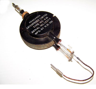 |
| The is the same type of 10 cm magnetron brought to
North America by the Tizard Mission in 1940. This specific example is Canadian Type 8 BX s/n 19152. It was manufactured by Northern Electric for Research Enterprises Ltd, a Canadian Crown Corporation. One of the filament leads is missing. |
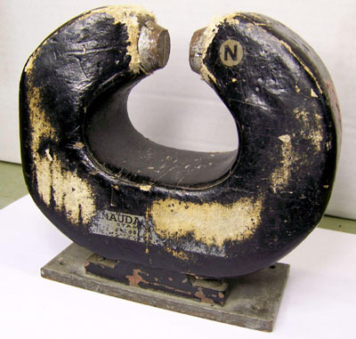 |
| This is the magnet for the magnetron. |
| (Both photos by Jacques Hamel, VE2DJQ, Le Musée Québecois de la Radio) |
The Germans captured a British magnetron in 1943, but it did not help their radar effort in a meaningful way. A substantial output of the German radar industry had to be devoted largely to fend off the Allied bomber offensive. Germany did have advanced radar technology at the start of World War II. In 1938, about one hundred FREYA systems were operational and were being used for aircraft detection and tracking. The FREYA operated on 125 Mcs with a peak power output of 15 to 20 Kw and had a range of 100 miles. Over a thousand units were built during the course of the war.German SEEKAKT radar was first installed on the Graf Spee and was used for surface search and gun ranging. It operated in the 120 to 150 Mcs band with a peak power of 8 Kw and had a range of 50 to 100 miles. About two hundred such sets were built, primarily for warships. The WURZBERG system became operational in 1940 and was used with gun batteries for anti-aircraft (AA) control. It operated between 553 to 566 Mcs with a peak power of 7-11 Kw and used a dish antenna with conical scan for precise aiming. The objective was to equip every AA battery with a Wurzberg. Over five thousand were built during the war.
Another advance in radar was duplexing, a method still in use today. This is a switching technique that allows the same antenna to be used for both transmission and reception by blocking the receiver during transmission periods. In addition, the echo signals are displayed on a CRT that uses a radial time-base that rotates in synchronism with the aerial. Since the targets appear in their correct plan positions relative to the radar station, this form of display is named the Plan Position Indicator (PPI).
The British were the first to conceive the filter centre, the room in which successive radar detections could be plotted and collated along with any other pertinent information. As an example, search radar presented the current locations of nearby aircraft. This is not what the decision maker needed. He was much more concerned with vectors (bearing, speed, and distance). A target fast approaching the ship, required a different response than a target that was passing by. The filter centres were eventually organized into units called the Action Information Centre (AIC) in the British Navy or the Combat Information Centre (CIC) in the US Navy, terms that still apply today.
These seaborne filter units would gather and collate information from several radars aboard ship and combine it with radar from other ships and intelligence sources. The output of the AIC or CIC complied a tactical picture that brought some order and sense into what was otherwise a very confusing situation. Remarkably, none of the Axis navies, all of which had radar in some form, seem to have created anything like AIC/CIC.
From time to time the AIC/CIC would become saturated. An example of this was the Japanese kamikaze attacks against US naval vessels. Now, the fleet was faced with so many individual targets that the CIC became saturated. As an interim solution, air control sectors were divided in such a way so that no individual CIC would become overwhelmed. Post-war experiments confirmed, however, that manual CIC's were quite limited. Eventually, this resulted in development of combat data automation systems using computers.
Radar in the S and X bands was also used as an aid in blind bombing missions to delineate the ground beneath the aircraft. It also functioned as a navigational aid as well as a target identifier. Microwave radars were also important to the anti- aircraft artillery units of the army, providing target detection and automatic firing of large calibre guns.
The great operational advantage of microwave radars during World War II was that they were relatively free from electronic counter measures (ECM) by the enemy. Electronic warfare has now become a major threat to military radar systems, and modern radars have to be hardened against ECM. For example, antennas have been developed with increased resolving power but with very low side lobes so that active jamming cannot penetrate the receiver as readily as with earlier systems. Additionally, the effect of passive jamming is reduced. The observation of false targets because of backscatter from chaff is also reduced considerably.
During the 1950's, radars had come to dominate the topside appearance of many ships. There were many of them, and they all competed for the few places that provided a wide arc of search. Some examples were air and surface search sets, pencil-beam sets capable of determining the altitude of a target and numerous fire control sets on top of the gun directors. Many ships were fitted with homing beacons that provided a point of reference for fighter control. Ideally, the number of radars could have been reduced by combining roles, but this was not practical with the technology of that time. Different operational requirements required different frequencies, pulse repetition rates, pulse widths, power levels and different rotational periods for antennas.
This short piece on magnetron use and care may be helpful to anyone who still maintains vintage sets. It was produced by the Royal Canadian Navy.
RCN FLEET TECHNICAL BULLETIN LE 02/18.
8 November, 1963GENERAL INSTRUCTIONS ON THE USE OF MAGNETRONS
Introduction
(a) Magnetrons are high-efficiency generators of microwave energy. In part, the high efficiency is due to the design, in that, the radio frequency circuits are actua1ly embodied in the anode (or plate) of the tube.
(b) This method of construction leads to certain limitations on the design. For example, to obtain increased power output from a magnetron at a given frequency, it is not usually possible to increase the size appreciably as is possible with almost all other types of tubes. The size of the anode block is dictated by the frequency at which the tube is to operate, and not only by the required power output.
(c) One result of the dimensional limitations is that in magnetrons, the current and power loading density is generally high. Magnetrons also have to operate at high voltages in order to obtain maximum efficiency.
d) Because of these factors, magnetrons are subject to certain limitations which have to be understood in order to obtain the best possible service from them.
2. Running Up a New Tube
(a) Magnetrons are largely constructed of metals such as copper, nickel, molybdenum and Kovar, an alloy of nickel, iron and cobalt. Glass or ceramic is used tor electrical insulation and in the output circuit for the transmission of the RF. output.
(b) One of the major problems during the manufacture of magnetrons is the removal of all gases which are normally absorbed in the, metal and glass used in the vacuum envelope. If these gases are not fully removed, the vacuum is poor and the tubes will arc internally. Even with the best manufacturing methods, it is not possible to remove all the gases from the inner layers of the . materials. These deeply absorbed gases tend to be liberated when the tubes are in storage and this causes a minute quantity of gas to be present in the vacuum envelope.
(c) The presence of this gas shows up in the form of internal arcing when the tube is first switched "on" in the equipment.
(d) Arcing can be recognized by a "flutter" on the voltage and current pulses, and by "kicks" in the mean current meter accompanied by simultaneous reduction of power output.
(e) Most magnetrons arc a little when switched "on" and in general, the arcing ceases after a few minutes operation. If a power level control is provided in the equipment, the output level should be raised gradually to operating value because excessive arcing may damage the magnetron..
(f) Slight arcing is not harmful and, indeed, is necessary so the gas may be 'cleaned up" thus permitting stable operation at the full output level.
(g) The power level control should be adjusted at a rate just sufficient to maintain slight arcing (say 6-8 kicks of the mean current meter per minute), whilst avoiding continuous arcing. Continuous arcing shows up as a substantial but fluctuating increase of the reading of the mean current meter. (The "mean" current meter is also called the "average" current meter.)
(h) When the tube is oscillating stable, the cathode heater current should be reduced in accordance with the instructions given in the Equipment Manual. (In many equipments, the reduction in heater current is automatic.)
3. Precautions To Be Taken To Ensure Maximum Life of the Magnetron
(a) Apart from the care required in starting a new magnetron, certain equipment maintenance jobs should be performed regularly in order to ensure maximum reliability of the magnetron in any equipment.
(i) Cooling of the anode is important and a regular check should be made to see that the blower, or circulating pump in the case of water-cooled tubes, is functioning correctly. Also make sure that the air filters and ducts are clean so as not to impede the air flow.
(ii) When the reduction of cathode heater voltage is automatic, a check should be made to see that the relay is operating correctly. An excessive heater power dissipation will damage the magnetron cathode. Heater connections should be examined periodically to see that they are free of corrosion and that good contact is made, otherwise, the magnetron will be starting with a cool cathode which may cause damage and reduce its life.
(iii) If in the particular equipment, the waveguide is pressurized it is important to maintain the required pressure. Reduced pressure may cause arc-over in the waveguide or coupler which may ruin the magnetron by cracking the glass. Also make sure that the cathode connector side arm is .kept clean and pressurized when facilities for this are provided.
(iv) If the magnetron is of a type which requires a separate permanent magnet, it is important to check that the magnet has the required field strength. If necessary, the magnet should be replaced.
(v) Magnetrons are designed to work into a feeder which has a voltage standing wave ratio less than 1. 5: 1. Care must be taken in the installation and use of the equipment to see that the V.S.W.R is kept at the lowest possible value.
A high S.W.R. may cause the magnetron to "mode" (misfire) and thus increase the cathode heating power, thereby reducing the magnetron life. A high V.S.W. R. can also produce malfunctioning of the magnetron, such as spectrum broadening or frequency jitter. These may not have any effect on magnetron life, but certainly degenerate the system performance. Any bent, dented or distorted waveguide sections should also be replaced, because they could produce an excessive standing wave.
(vi) Modulator performance also has an important bearing on magnetron life. Certain modulator faults can cause pulse distortion which could impair magnetron life.
(b) It is important to see that the "overswing" or backwash diode is operating satisfactorily. Loss of cathode emission in these tubes can cause excessive magnetron arcing by allowing greater than normal voltage pulses to be developed.
(c) A spike at the beginning of the voltage pulse is very undesirable. It can increase arcing and can also cause mode change.
4. Failures
(a) The common causes of failure (with symptoms) are listed below. This should help the user to diagnose the cause of failure.
(I) Down to Air" - It is possible for the glass or ceramic parts of a tube to crack and thus admit air into the magnetron. A tube which is down to air will take excessive magnetron mean current, show a blue glow internally, and have a much reduced voltage pulse. There will also be no power output. Running the heater for any length of time in an air-filled tube will lead to heater burn-out.
(ii) "Low Power" - The output of a magnetron falls during its life and most magnetron lives are terminated by this cause. The symptoms are generally only low power as measured on the power monitor and weak echoes on the display system.
(iii) "Low Pulse Voltage" - Sometimes the pulse voltage of the tube falls and this results in unsatisfactory operation. Low voltage also means low power output and can be detected by measuring the pulse voltage on the monitor oscilloscope.
(iv) Open Circuit Filament - No heater? current will be drawn by the magnetron. The filament side arm will feel cold and the magnetron will not start oscillating. There will be no power output and also an excessive voltage pulse. Filament voltage will be greater than normal because current will not be drawn from the transformer.
(v) "Short Circuit Filament" - Excessive heater current will be drawn by the magnetron. The filament voltage will be low and the tube will not oscillate. The pulse voltage will be higher than normal because no anode current is drawn.
(vi) "Excessive Arcing" - It is possible for the magnetron to arc continuously so that radar performance is impaired. In some tubes arcing increases as the end of the life is approached. It is up to the discretion of the operator to determine the moment when the arcing is sufficient to warrant removal of the tube from the equipment.
(vii) Mode Change - In some types of magnetrons the cathode emission fails after some hundreds of hours of life. This may have the effect of causing "mode" change. Mode Change can be recognized by the fact that double traces of voltage and current pulses are viewed on the monitor. There will also be missing 1ines in the spectrum since during those pulses when the magnetron operates in the wrong mode, the output is much reduced and is at another frequency.
(b) In many cases, incorrect magnetron functioning is caused by equipment faults. It is therefore important to look for equipment faults (such as pulse transformer breakdown, modulator misfiring, bad connections etc). This may cause magnetron failures in quick succession.
5. Special Note
(a) Some types of' magnetrons do not give their full output when first switched. "on" after a period of storage.
(b) When checking a new tube in a transmitter, allowance must be made for this effect which is due to a small reduction in cathode emission.
(c) Normally, a few minutes of operation will restore the emission and full output will be obtained with a clean spectrum, but in the case of operation at very low duty ratio in relation to the JAN specification, it may take thirty to ninety minutes before full normal operation is re-established.
Signed
(J.N. Doull)
Commodore RCN
Director General Support Facilities.
This section will summarize radar systems used by the RCN in the 1940's and beyond. This is not a complete listing. Comprehensive references can be found in "Naval Radar" by Norman Friedman or "Development of Radar in the Royal Navy" by Alastair Mitchell.
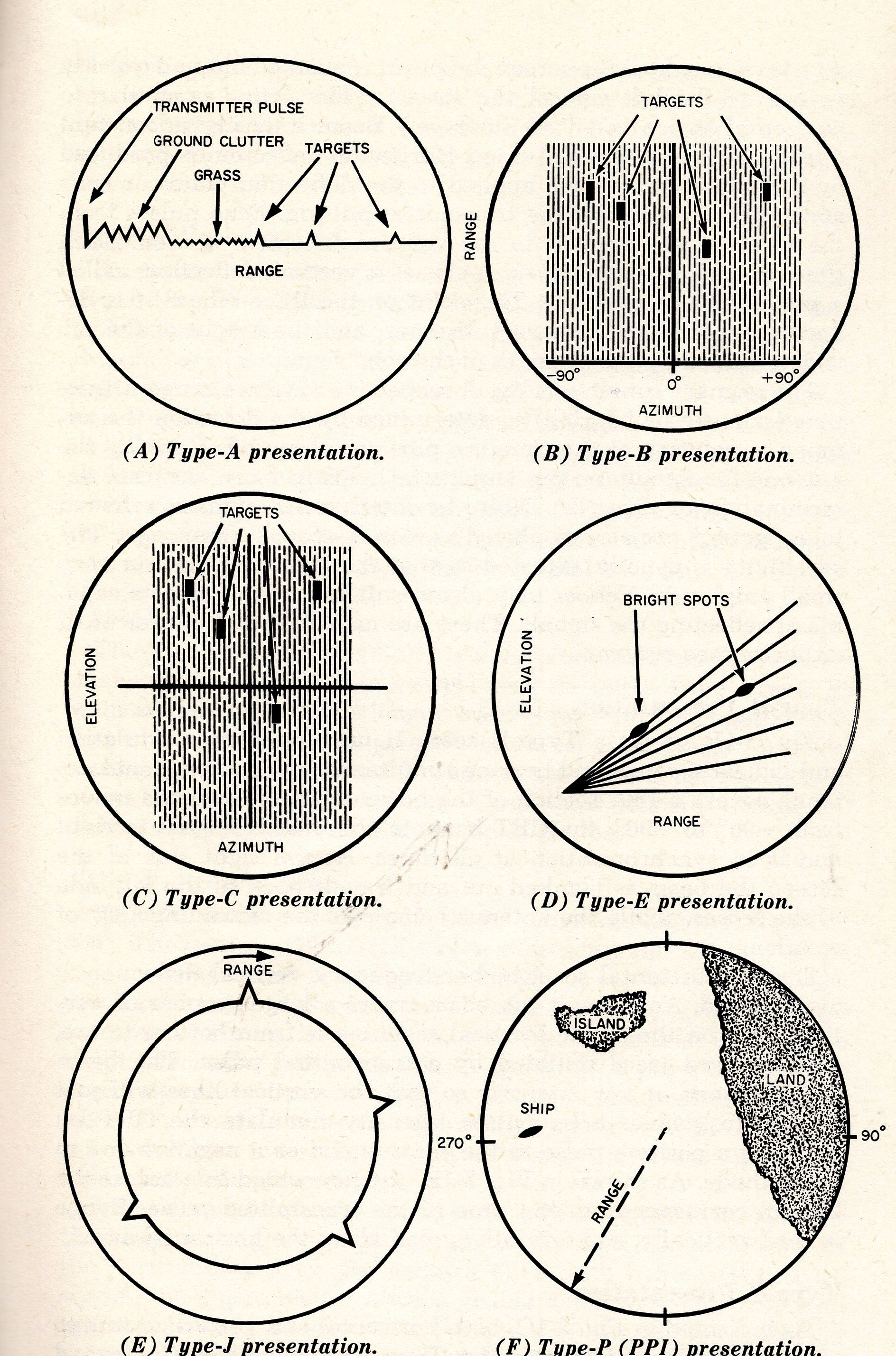 |
In the equipment descriptions which follow, the
most common display types mentioned are the "A" display and the "PPI" type.
Other less common displays can be seen by clicking on the image. (From ABCs of Radar) |
HMCS HAIDA RADAR and RDF FITSThe former acronym for radar was RDF which stood for Radio Direction Finding/.
1944 - Foremast top: 291 combined.
After boathouse: 271 combined with 241 IFF pitchfork antenna.
Mainmast: HF/DF birdcage antenna.1948 - Foremast top: HF/DF birdcage.
Foremast midpoint: 293 'cheesecake'. ( May have been installed during HAIDA's 1944 Canadian refit)
Mainmast: 291 combined.1953 - Korea, first tour of duty.
Foremast top: 293 WC type. (Warning Combined.
Descending order: IFF dipole; Sperry HDWS radar (Mark II)
Mainmast stump: 291 combined.1954 - Korea, second tour of duty.
Foremast top: 293 WC type. (Warning Combined.
Descending order: IFF dipole; AN/SPS6C; Sperry HDWS
Mainmast: 291 combined (rarely used).1956 - SHF/DF antenna added to foremast top for AN/UPD501 radar DF set.
CSC means Canadian Sea Control type and was the prototype for the SW1C set. As completed, the CSC consisted of two separate cabinets. The first contained the transmitter and power supply while the second cabinet housed the receiver and a five inch CRT that presented information in 'A' scope display. It operated at 200 Mcs or 1.5 meters, a frequency chosen specifically to avoid interference with 286 sets.Two major design compromises were made in order to get the prototype to sea on schedule. One concession was to use a transmitter of lower power than original design specifications due to the unavailability of certain vacuum tubes. The second compromise was to use a fixed antenna system similar to that of the 286. Sea trials of the CSC set began in HMCS Chambly using a Dutch submarine O-15 as a target. All tests indicated that the system was successful as the submarine was spotted at 2.7 miles. On this basis, the RCN Naval staff agreed to proceed with the fitting of the CSC in all ships but they did not know that the test results were flawed.Apparently, the Dutch submarine was fully surfaced when detected, but German U-boats developed the tactic of running in a trimmed down mode. Admiralty tests indicated that the best range obtained on a 286 set for a trimmed down U-boat was 1.5 miles. All of this went unnoticed by the RCN who in, turn ordered the set into production as the SW1C.
When World War II broke out, there was no radar industry in Canada and any requirements for naval radar had to be filled by the British. This was not considered a satisfactory arrangement, therefore the National Research Council in Ottawa started development on the infamous SW1C (Surface Warning 1st Canadian) radar in 1941. This system saw its service debut in RCN ships starting in 1942.According to many who used it, the SW1C was considered a menace. A target on the starboard bow could just as well be on the port quarter. Practical experience indicated that the set had a propensity to generate false echoes and the long pulse of the set meant that it could detect nothing within a half mile of the ship. This level of performance from the system did not instill confidence to those who had to operate it. Part of the blame can be assigned to the scientists who failed to design a sailor and sea- proof set and the RCN which trained operators and not maintainers. By the time the RCN began to look seriously at the need for qualified radar personnel, the country had been stripped of them in order to support the high-tech air war in Europe. As late as 1943, the navy had to draft RCAF radar technicians for its corvettes in order to keep the radars running.Quite apart from numerous U-boat contacts that went unnoticed in the clutter of echoes displayed on the glowing CRT, the set was the active cause of many serious accidents and collisions, putting some ships aground and ramming others into other unyielding objects. It was infuriating for the Officer of the Watch to vainly search for objects reported by the SW1C only to have something large and substantial go streaming by and then discover that the operator did not detect it on his wretched set. As an example, off the coast of Labrador, on a clear sunny day, it might detect a tiny piece of floating slush at an amazingly long range, and at midnight it would fail to detect an approaching iceberg.
Due to poor liaison, the RCN never realized that the Royal Navy had already introduced a superior new generation of radar (271 type) in 1941. Ascertaining why the Canadians got off to a late start requires some speculation, since the documentary evidence is incomplete. It is significant that the decision to opt for the SW1C was made prior to large scale RCN involvement in anti-submarine warfare. As a result, SW1C was obsolete in its primary role as a submarine detector before it entered production and the RCN committed to its production for at least a year after 271 entered service. Due to this commitment, the RCN, for the rest of the war, was unable to provide the timely supply of sufficient centimetric sets for its own growing escort fleet. In spite of being given the highest priority rating, production of the SW1C was delayed due to the shortage of small motor-generators and vacuum tubes. By the last week of 1941, only fifteen corvettes and three merchantmen were fitted with the CSC and SW1C. A few sets were provided to the RN in June 1941. One set was fitted aboard HMS MALAYA.
From Friedman' book NAVAL RADAR, the expected performance of the SW1C set:
Detection of -
* Surfaced submarine - 3,000 to 4,000 yards
* Corvette - 5000 yards
* Cruiser - 14,000 yards
* Aircraft out to 25000 yardsAt one time HMS MALAYA detected a Swordfish aircraft at 500 feet altitude at 20,000 yards. Accuracy was 4 degrees and 200 yards but an accurate range was impossible inside 1000 yards.
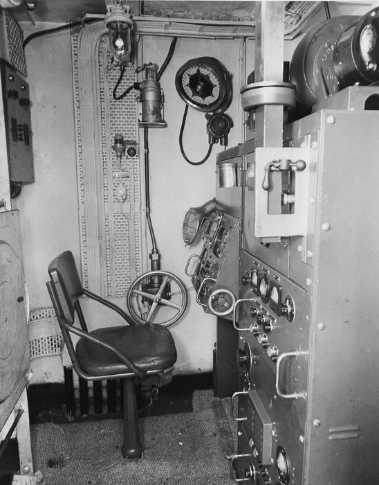
The SW1C antenna consisted of a rotating, multi-element, Yagi antenna. It was also ironical that this antenna was invented by a Japanese physicist. When used in a radar applications, Yagi antennas are susceptible to detecting targets on reciprocal bearings, hence one of the reasons for the unreliability of the system. Rotation was provided by a rather cumbersome and primitive mechanism composed of a steel shaft connected to a sprocket and chain reduction gear, which in turn, was rotated with, of all things, a Chevrolet steering wheel mounted in the RDF office! On every ship that was fitted with SW1C, this arrangement became known as 'the plumber's nightmare'.
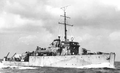 |
| The SW1C Yagi antenna can be seen atop the mast of HMCS Wasaga, a Bangor class mineseeper which served in the RCN from 1941-45. (Photo courtesy Naval Museum of Manitoba) |
The SW1C Yagi antenna can be seen atop the mast of HMCS Wasaga, a Bangor class mineseeper which served in the RCN from 1941-45. (Photo courtesy Naval Museum of Manitoba)Repeated failures of the main rectifier tube continued to plague the set, but modifications were made to replace the tube with an improved model. Beam accuracy was also improved to within 5 degrees and more importantly, bearings were possible over a 360 degree arc. This was a major improvement over the Admiralty's 286 set whose accuracy and directional search was limited by its fixed antenna.
The transmission line between the set and the antenna was saturated with nitrogen gas to reduce signal attenuation. It proved to be a cumbersome arrangement that caused major headaches from January 1941 until the end of its service life in 1943. A recurring failure of a co-axial cable seal allowed sea water into the cable, which in turn, introduced losses and attenuated the signals to the point where it rendered the set almost useless. The stresses and strains of rotating a mast-top aerial were extreme, especially when effects of high winds, severe winter icing, and the ship's movements were taken into account. Adding to this, was the requirement to purge the co-axial cable at periodic intervals. Of course, the gas bottle that performed this task was fitted in the operator's cabin, but the valve to open and vent the line was located where else -- but at the top of the mast. Climbing aloft to purge the line during a midnight blizzard was an experience that must still haunt former RCN radar operators. One rating actually stood on the wheel house roof throughout a Cape Cod blizzard rotating the broken antenna by hand with a Stillson wrench while the ship groped through an oncoming convoy. He was rewarded and revived by five successive hot buttered rums in the wardroom upon arrival.
Regardless of the problems, production of the set continued into 1942. The first major model change was the conversion of the SW1C to 214 megacycles to make it compatible with Identification, Friend or Foe (IFF) sets and additional improvements to the Yagi antenna. This re-designed set was known as the SW2C and formed the bulk of the units fitted on corvettes and minesweepers.
 |
| The SW1C radar installation aboard HMCS MONTREAL K319 taken on February 7th, 1944. MONTREAL was a River Class Frigate. (Public Archives Canada photo HS-0410-16 submitted by Spud Roscoe) |
In later productions, the SW2C set was modified for use on small ships such as Fairmiles and motor torpedo boats and was renamed the model SW3C. The major difference was a modified Yagi antenna that was lighter and slightly different in design. This variant entered service in mid-1942. Until ten centimetre radar equipment became available in large quantity in mid-1943, the SW series was the only radar available to the RCN in great quantity. Long after the Admiralty had removed the 286 from service, the SW2 was retained by the RCN for aircraft detection and a reserve set. The decision made by the RCN to continue production of the SW1C made sense at the time as it was next to impossible to procure 271 sets in great quantity.When centimetric radar entered widespread use in the autumn of 1943, the Royal Navy Western Approaches Command tried to persuade the RCN to remove the SW series set from its vessels since it was deemed a maintenance nuisance. The SW2C was defended with vigour by most Canadian operational commanders and Naval Staff who not only wanted to retain them, but improve them as well. This attitude led to the design of the SW2C/P and the SW3C/P sets that had a defect- free antenna and a PPI display. This permitted the SW series to continue in service until the end of 1943.
In spite of much pro-SW2C attitude from officers and others, that radar type was not being maintained in ships where it co-existed with type 271. In fact, Canadian Confidential Naval Order Number 188 dated May 29th, 1943 was issued to address the situation. It read as follows:
"Information has been received that some ships which are fitted with both type SW2C and type 271 radar are neglecting the maintenance of the SW2C. It should be realized by Commanding Officers that the SW2C set is a valuable piece of equipment operationally both as an aircraft warning set and as a standby for type 271.
Steps are to be taken to ensure that SW2C is at all times ready for effective use and that the RDF cabinet is not used as a storage space for other gear"
Regardless of the faults of the SW1C, RCN officers managed their battles with much less information than their British counterparts -- a situation that called for exceptionally high standards of co-ordination, leadership, training and seamanship.
According to Norman Friedman, 'Naval Radar' (USNI, 1981), pp. 201-2: "SW-1C: This Canadian radar was installed in several US and British warships early in World War II, the largest beingHMS 'Malaya'." He doesn't cite which USN ships.
| Select this link for SW2C photos |
267MW The 267MWradar is cited in BRCN 213 (circa 1960) , the RCN's Materials Catalogue. This may be a submatine radar circa 1945. No further info found at this time.
This was an X-band (3cm) surface search and navigational radar developed in Canada for the British Admiralty in 1944 with initial fittings aboard Motor Torpedo Boats. Later it was installed on Algerine class minesweepers, Hunt class Escorts and Coastal Forces Craft. The main design goal of this radar type was to locate U-boat schnorkels. When first developed, the RCN knew of the type 268 but its small antenna and resulting short range limited its value for escort work. The British were aware of the problem and had developed a larger, more powerful antenna for the system. This exclusively British development became the 972 set. Most of the 268 sets were fitted during the period 1945-52 and they were later replaced by the Decca Type 974.Power output of the 268 set was 30 kw at a frequency of between 9320 and 9475 Mcs. The antenna was a 30" half cheese type producing a beam 2.5 degrees by 17 degrees. It rotated at 22 rpm and there was no stabilization. A PRR of 500 permitted detection of a battleship at 9 nm and a submarine at 3 nm.
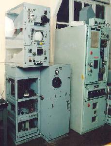
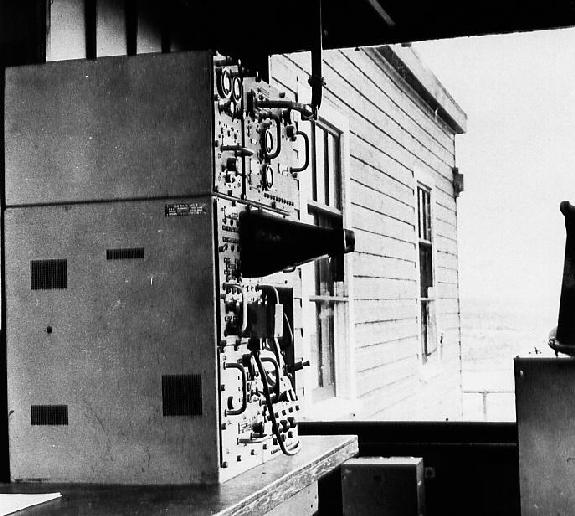 |
| The 268 radar set at Radio Camperdown VCS as it appeared in September 1949. (Photo courtesy National Research Council #2360C. Submitted by Spud Roscoe). |
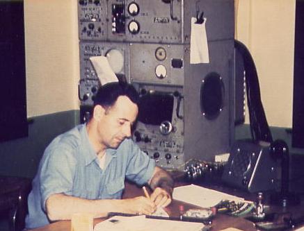 |
| David Clarkson is at the Radar Plotting Position Camperdown Radio VCS in 1956. Behind him is the 268 radar. (Photo by Alex Murray submitted by Spud Roscoe) |
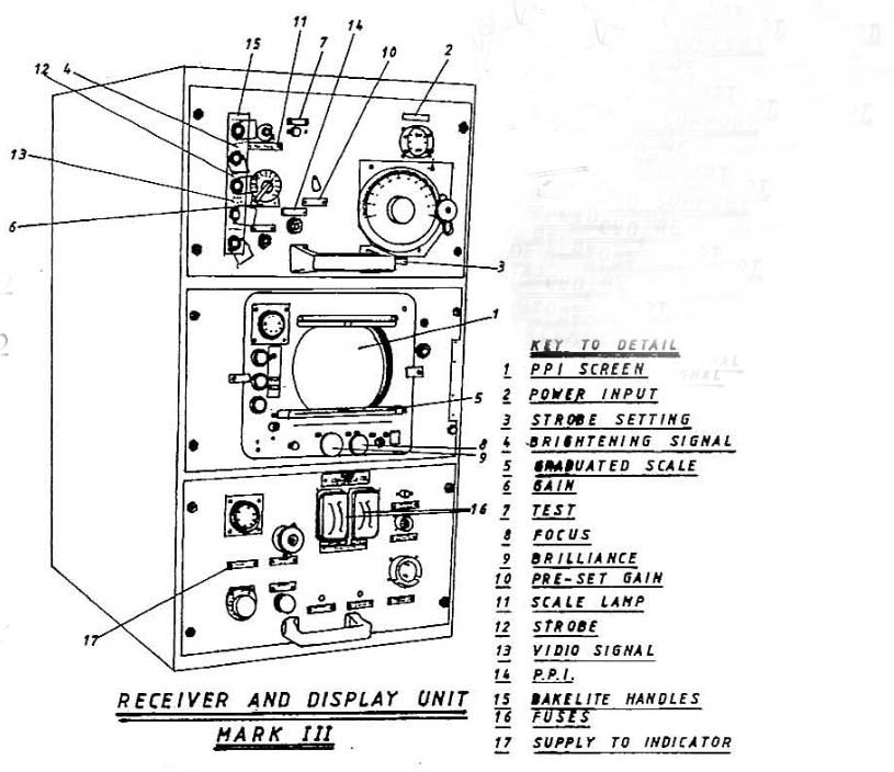
 |
268 radar basic components. Click on thumbnail to enlarge. (From the 268 radar manual) |
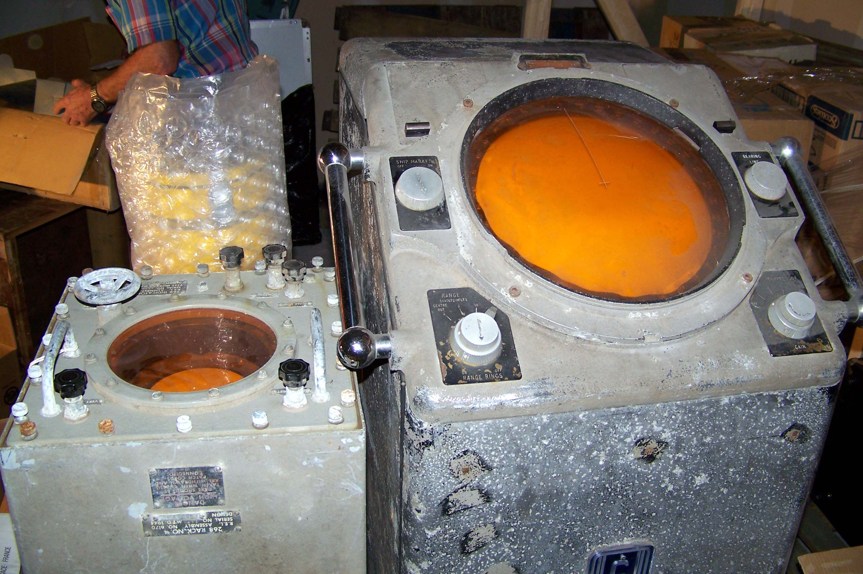 |
| Wheelhouse Indicator is at the left and the Console Indicator is at the right. |
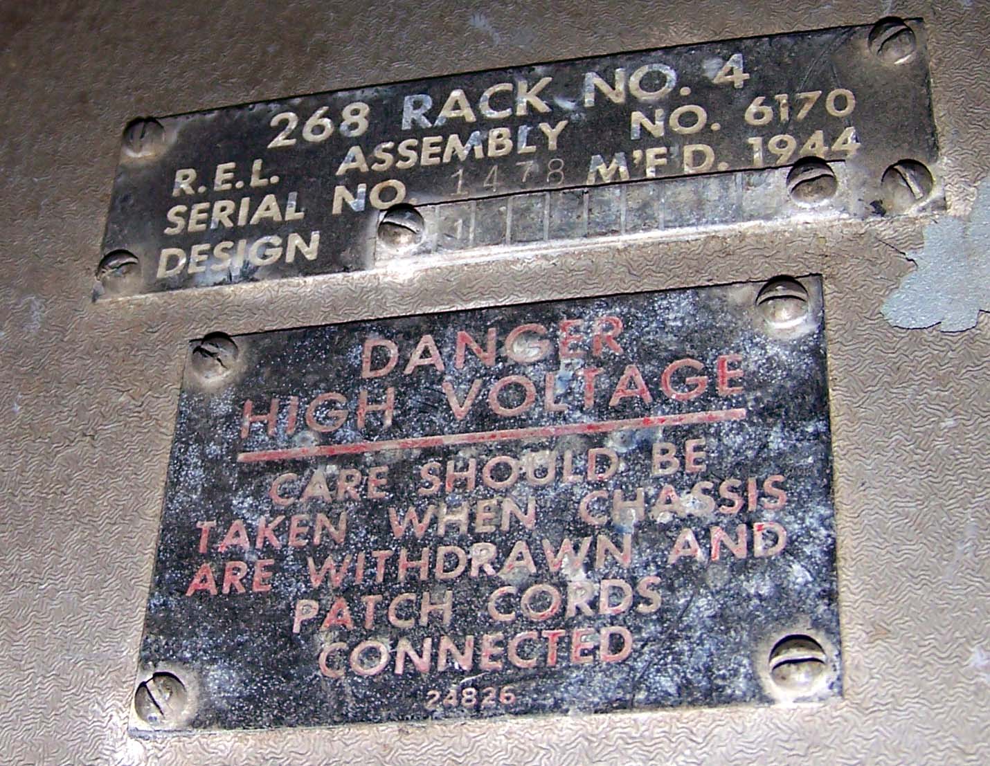 |
| Rack 4 (repeater) nameplate. |
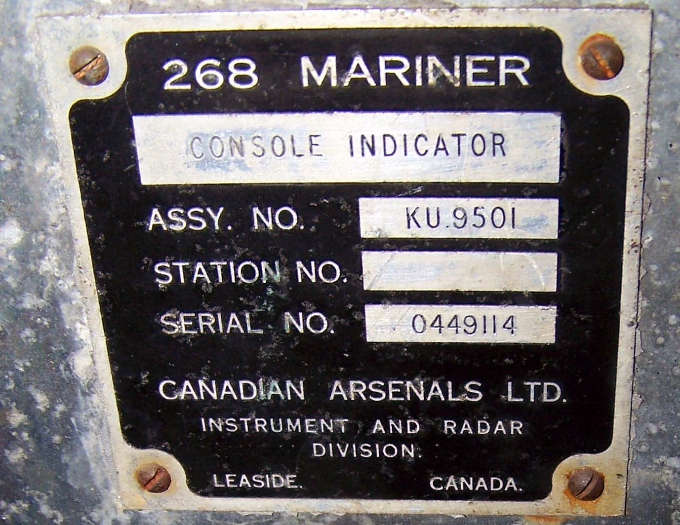 |
| Nameplate found on console indicator. |
| Photos in thi table courtesy Le Musée Québecois de la Radio |
| KEY 268B SPECS FROM MANUAL | |
| PARAMETER | VALUE |
| Frequency Range | 9345 to 9405 MHz |
| Maximum range | 60,000 yards in 3 ranges: 6,000, 30,000 and 60,000. |
| Minimum range | 80 yards. |
| Range resolution | 100 yards |
| Bearing resolution | 2 degrees |
| Peak Power output | 30 kilowatts |
| Duty cycle | .0005 |
| Pulse width | 0.75 microseconds |
| Pulse repetition rate | 500 Hz |
| RF generator | 725A magnetron |
| Horizontal beamwidth | 2.5 degrees between half power points |
| Vertical beamwidth | 11 degrees between half power points |
| Receiver IF | 31 MHz |
| Indicator | 5 inch PPI |
| Antenna | Parabilic cyliner |
| Antenna rotation | 22 rpm |
| Transmission line | Waveguide |
| Supply voltage | 110 or 200 VDC |
| Maximum power draw | 2 kilowatts. |
271 TYPE
While the SW1C prototype was being tested in HMCS Chambly, a new air/surface warning set, namely the 271, was being tested aboard a Flower class corvette, HMS Orchis in England on 25 March 1941. The 271 set, using the cavity magnetron, operated on ten centimetre wavelengths (3030 MHz) at a power level of 5 kilowatts, was keyed by 1.5 microsecond wide pulses at a PRF of 500 Hz. This was quite a breakthrough in technology for the time, however it only used a ranging display (A scope), a rather inefficient means for a search radar. Its finer and narrower beam (5 degrees H by 20 degrees V) would permit escorts to detect trimmed-down U-boats at long distances, consistently and accurately. Sea trials indicated that the 271 could detect a trimmed-down submarine at 3,500 yards and a periscope at 900 yards. A battle ship was detectable at 13 nm. This was a sharp contrast to the unrealistic test results of the SW1C.After the British provided a "gift" magnetron to the USA in November 1940, progress there was also very rapid. The Type SG set designed by Raytheon went to as a prototype in a destroyer with a display using a Plan Position Indicator (PPI) in June 1941. The SG worked on a frequency of 3175 MHz with a 50 kW output.
By the spring of 1943, the large majority of mid-ocean escorts were fitted with the 271, however, many ships of the Western Local Escort Force were not. To complicate matters, the British introduced two improved models, namely, the 271P and 271Q. Both of these versions had output power increased from 5 kilowatts in the 271 to 90 kilowatts in the 271Q. This quantum jump in power output can be directly attributed to a major improvement in magnetron technology. While the RCN was struggling to fit new ships with first generation 271's, they were also under great pressure to upgrade existing radars. By September 1943, only fourteen 271Q sets and fifty three 271P's were fitted into RCN vessels along with three original production models. The introduction of 10 cm radar into fleet destroyers was delayed until the needs of the escorts were satisfied.
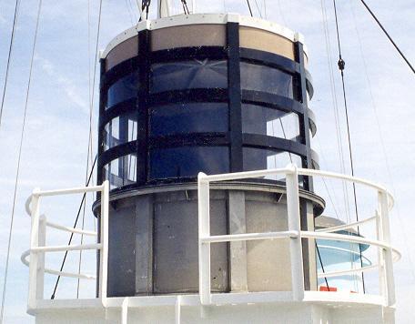
Since the 271 set operated at the 10 cm wavelength, the antenna could be made small enough to be housed in its own Perspex bubble and mounted on top of the operator's cabin. The antenna consisted of a 'double cheesecake' with separate transmitting and receiving antennas stacked one on top of the other. This radar was sometimes called 'lighthouse' due to the shape of the dome. Some of the transmitting and receiving elements had to be affixed directly to the back of the antenna to overcome co-axial line losses. In the original 271, the power feed to the antenna was by coaxial cable so this limited rotation to 200 degrees. When the original magnetron was redesigned to produce higher power, waveguide was introduced to the antenna system. Coaxial cable could not handle those power levels.
Initially, the new 271 set was viewed with suspicion by the crews of the ships in which they were installed. Noting that the ratings were reluctant to go aloft, especially to the crow's nest just above the 'lighthouse', the captain of a ship in which a new 271 radar had just been installed questioned a seaman as to the reason. After a bashful amount of toe stubbing, the sailor confessed that the 'buzz' was that rays from the set would make a man impotent. Nipping an incident in the bud, the quick witted captain declared the rumour to be nonsense. "Radar rays", he maintained, "made a man temporarily sterile, not impotent". From this viewpoint, it was viewed as a bonus rather than a drawback especially on shore leave. The 271 then radar became the most popular piece of equipment in the ship.
A 271 set was installed on HMCS Haida during her January 1944 refit while she was in Plymouth. The radar hut was located astern between the searchlight and the pom-pom guns. An integral, perspex, "hat-box" antenna was mounted directly above the 271 office.
Perspex enclosure for the 271 radar antenna. This is the recreated enclosure found on HMCS Sackville. (Photo by Jerry Proc) Mockup of a 271 radar console aboard HMCS Sackville.(Photo by Jerry Proc)
 |
| Description of the controls for the 271 radar, (Source not known) |
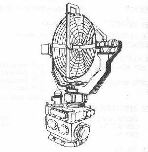
271 antenna front view. Click to enlarge. There were two, cheesecake style parabolic reflectors mounted on top of each other. One was for receive and the other for transmit. The antenna was manually trained by a handwheel in located in the radar office. (Image source unknown)
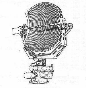
This is a rare image of the 271 radar antenna backside. (Graphic source unknown)
 |
| 271 Radar Installation . (Photo courtesy of HMS Collingwood, Fareham England) |
275 TYPE
Michael Young of Nepean Ontario lends his expertise to explaining the 275 radar fit aboard Tribals. "HMCS Cayuga (DDE218) and HMCS Athabaskan (DDE219) were the only Tribals not fitted with the 4.7" gun on-build. Instead, they were fitted with 4" guns and the dual purpose (surface and air) Mk 6 Director which had the radar antennae mounted on either side of the director like searchlights. One was the transmitter antenna and the other the receiver. The radar was the 10 cm type 275. At the time, this was the most modern system available. It had been developed as the director for secondary armament in cruisers and RN Battle class destroyers but also saw service in Darings and other classes of ships. 275 was eventually replaced by the MRS series in the Royal Navy.
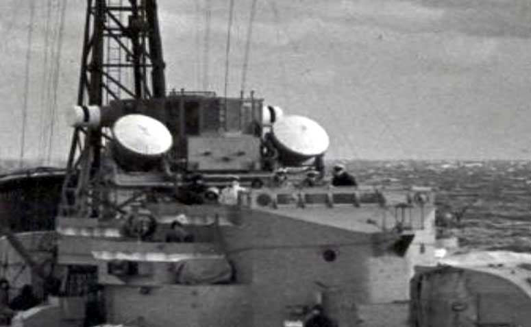 |
| HMCS Cayuga showing her 275 radar fit. (RCN Photo) |
The ASW conversion of the Canadian Tribals between 1951-55 introduced the USN GFCS 63 into all but DDE218 and DDE219. They kept the Mk 6 system. For surface fire, a stripped down version of the Mk III (W) director was fitted to complement the 63 since the 63 system was designed to knock down the Kamikaze! There was not much more modern stuff available before the Tribals came to the end of their useful life in the early 1960's that would have made further investment of any value".275 radar provided range, bearing and elevation, a full tachymetric fire control system and full blind fire high angle capability.SPECIFICATIONS:
Year: 1944-45
Frequency band: 3100 MHz
Power output: 600 Kw
Pulse width: .5 us
Range: 30,000 yards
Accuracy: 10 minures of arc in both planes.
Antenna: Two 4 ft. diameter parabolic dishes in nacelles either side of MK6 director. Separate receive/transmit dishes used with receiver offset to produce conical scan when spinning.
 |
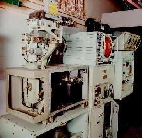
275 radar sysytem. Click to enlarge. The fire control tables are not shown in this photo. (Courtesy CB 4182/45 Radar Manual via Øyvind Garvik ) |
A surface search radar, the successor to 272 and briefly fitted in some destroyers in 1943-44. It was produced only in limited numbers, for ships which could not take Type 277, and postwar it gave way to Type 293. It introduced the 500 kW S-band transmitter operating with 1.5- and 1.9-microsecond pulses at a PRF of 500, with an alternative short-pulse mode of 0.7 microseconds, which characterized Types 277, 293 and 980 through 983. The antenna was a single power rotated 'cheese' stabilized in azimuth (outfit AUS) driving both A-scope and PPIs, scanning a 0-15 rpm with a 3.5 deg beam. Typical ranges, with an antenna height of 70 ft, were 16nm on a battleship, 14 on a cruiser, 12 on a destroyer, 10 on a corvette, 7 on an MTB and 5 on a submarine. Aircraft at 200-6000 ft could be detected at 13-17 nm. Range scales were 15,000 yds (accuracy 50 yards), 75,000 yards (250) and 150,000 yards (500).
Type 277 was a 10 centimetre surface/low air search set introduced into naval service in 1944. Sometimes it's described as the most successful wartime British naval radar. Using 500 kilowatts of power and keyed by 1.5 microsecond pulses, its 4.5 degree by 4.5 degree beam could detect a battleship at 23 nm. Type 277P could detect an aircraft between 5,000 and 20,000 ft at 55 nm. Post war type 277Q was generally fitted with 293Q.
 |
| 277 radar installation. (Photo courtesy of HMS Collingwood Chide, Fareham England) |
 |
 |
| 277P uses aerial outfit AUK. It was stabilized in both elevation and azimuth and producing a 4.5° x 4 .5° beam. (Image courtesy British Admiralty) | The post-war 277Q used aerial outfit ANU. This clipped parabola produced a 4.5° x 2 .5° beam for more precise height finding. (Image courtesy British Admiralty) |
|
|
|
 |
277 Office. Click to enlarge. 1 - PPI Display; 2 - 'A' Display; 3 - HPI display; 4 - Aerial bearing indicator. Click to enlarge. (Courtesy CB 4182/45 Radar Manual via Øyvind Garvik ) |
 |
277 Aerial Outfit 'AUK' Click to enlarge. (Courtesy CB 4182/45 Radar Manual via Øyvind Garvik ) |
281 TYPE
In 1941, the 281 air search set was developed and it operated on a wavelength of 3.5 metres. It was the principal British wartime air search radar for heavy ships. It's 350 kilowatts of output power was keyed by pulses that were 12 microseconds in duration. The antenna produced a 35 degree beam horizontally and vertically and a bomber flying at distances of up to 115 nm could be detected with this system.
 |
| 281B radar. Items in this view:
1 - PPI display 2 - 'A' displays 3 - Accurate ranging 'A' display (now obsolete) 4 - Aerial bearing indicator 5 - Aerial training control hand wheel. (Photo courtesy CB 4182/45 Radar Manual via Øyvind Garvik) |
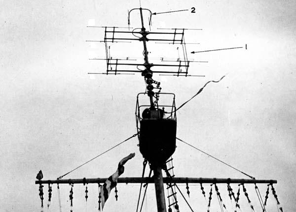 |
| Item #1 - 281 antenna. Item #2 Type 243 IFF interrogator antenna. (Photo courtesy CB 4182/45 Radar Manual via Øyvind Garvik) |
285/285P TYPE
This was a secondary-battery gunnery radar, first built in 1940 and then fitted in 1941. It employed two types of aerials; one with 6 Yagi's and the other with 5 Yagi's. In the six Yagi version, three aerials were used to transmit and three to receive. This arrangement produced a narrower 18 by 43 degree beam. Bearing accuracy was 3 to 4 degrees typical, with an accuracy of 100 yards on the 15,000 yard scale. This 25 kilowatt set was keyed by 1.7 microsecond pulses and operated at a 50 cm wavelength. At maximum range, it could detect a cruiser at 7 nm. On Haida, the 285 set was fitted-on-build (1943). The gunnery office was located at the base of the foremast while the aerial was mounted atop the director control tower on the bridge. The 'P' variant was an improvement on the original design with the introduction of a transmit/receive switch (T-R) which permitted the use of a common antenna. Beam width was reduced to 9.5 degrees along with a reduction in pulse width and higher transmitter power. The Auto Barrage Unit (ABU) which was associated with the Ranging Panel L22 was also installed. ABU was fed with range and rate of change information from the L22 panel and using a mechanical calculator, provided the 'instant of fire' for range settings on the fuzes in use.Unfortunately, the 285 was fundamentally flawed due to its inability to follow aerial targets in elevation and was replaced with the model 275. As the director was manually controlled, it was difficult to follow fast moving aircraft.
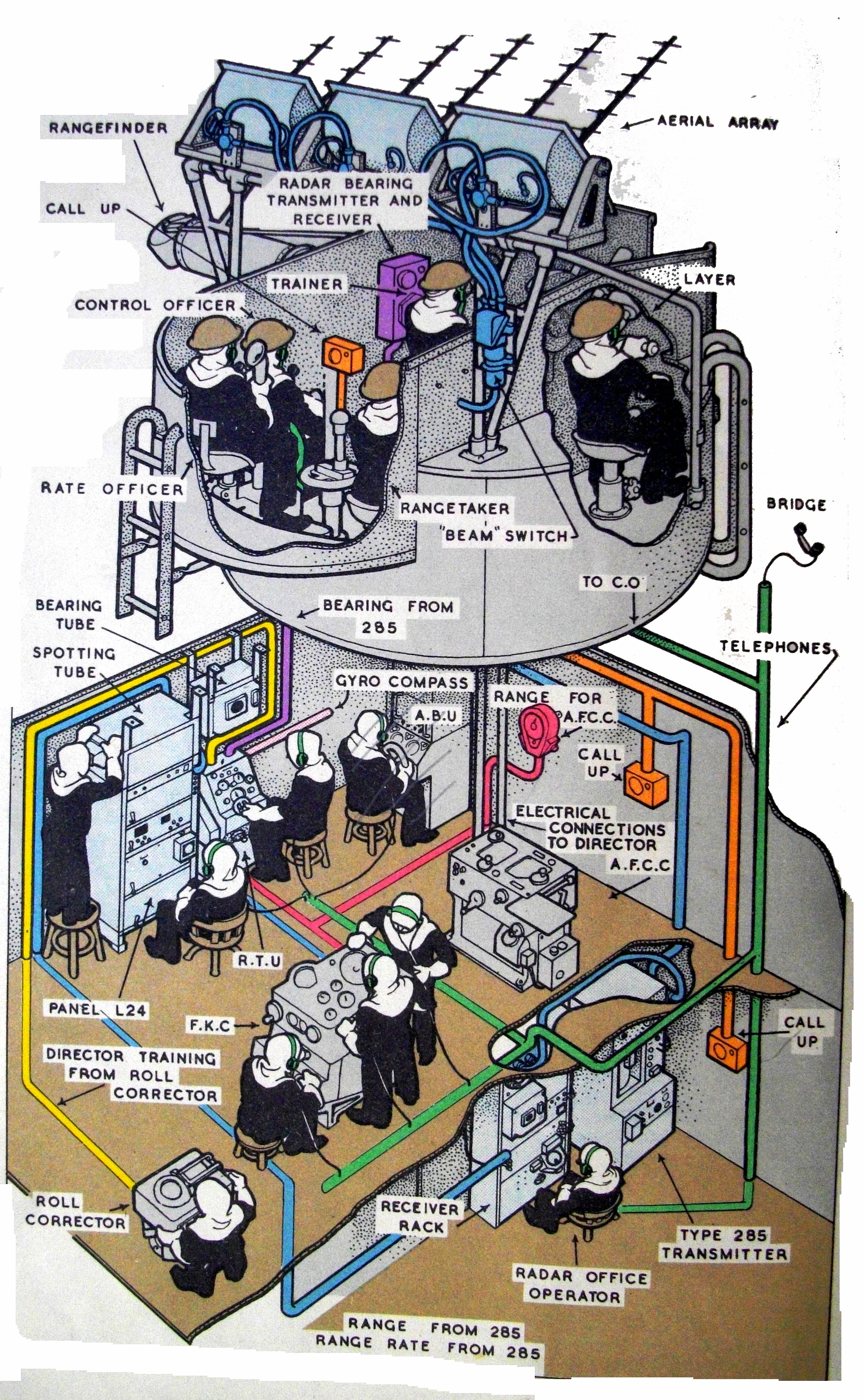
The most important information aboard the 285 radar is the fact that the Fire Control system came in two configurations. The first is the High Angle Control System (HACS) which was usually fitted on battleships and cruisers. The second system was the Fuze Keeping Clock (FKC) which was fitted on smaller ships like destroyers. Examples of these configurations are shown below.
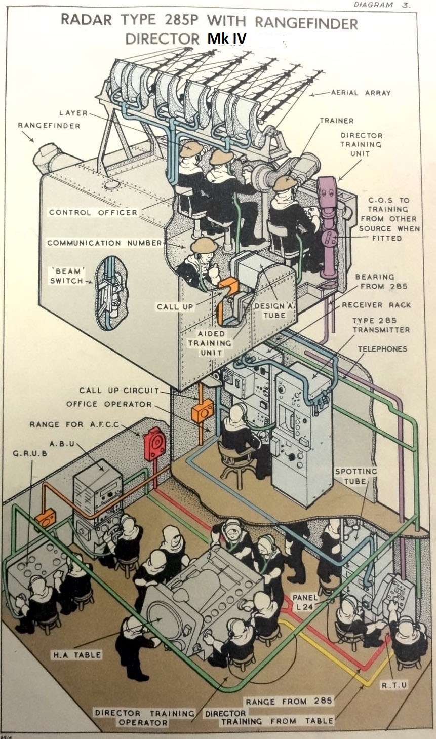 |
| The High Angle Control System. (HACS) with a Mk IV rangefinder in this example. (From BR1634) |
 T T |
| A 3D view of the FKC (Fuze Keeping Clock) configuration. (Royal Navy) |
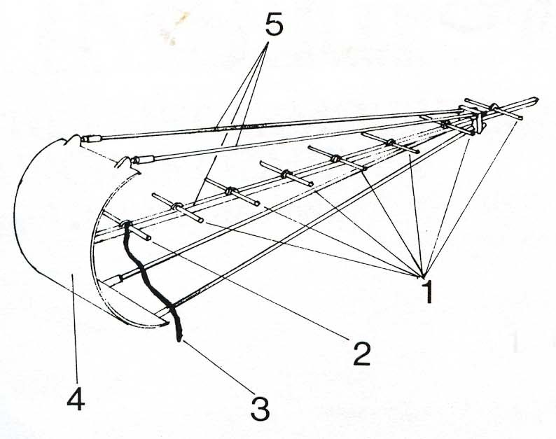 |
| Close-up view of a single Yagi antenna. There were six of these mounted
atop the 3W rangefinder. Three were for receive and three for transmit.
#1 - Passive element (aka director). #2- Driven element ( active transmitting dipole) #3 - Feed line to active dipole. #4 - Reflector element #5 - Non metallic supports. In British slang, the Yagi was referred to as a "fishbone " antenna. The Yagi antenna was named after the Japanese radio scientist who invented the antenna |
John Wise explains the beam splitter function of the 285 radar." Early fire control radar employed simple pulse and scanning structures that did not permit auto tracking. Within a short time a transmission process known as beam switch was introduced. There are two forms but for the purpose of explanation their result is the same. A pulse is transmitted and two adjacent receiver channels detect the returning echoes. If the two channel have balanced amplifiers and both indicate the same gain, on a CRT, for a given input signal, then the radar antenna must be looking directly at the target and that information can be used to slave a gun onto the same bearing. If, however, one input signal is higher than the other, the higher gain channel must be closer to the true target azimuth. This difference data can be used to auto correct the antenna tracking , which the slaved gun can follow. If the auto aspect fails for whatever reason, then the radar tracking operator uses the visual CRT clues to manually track and the gun can still follow".
 |
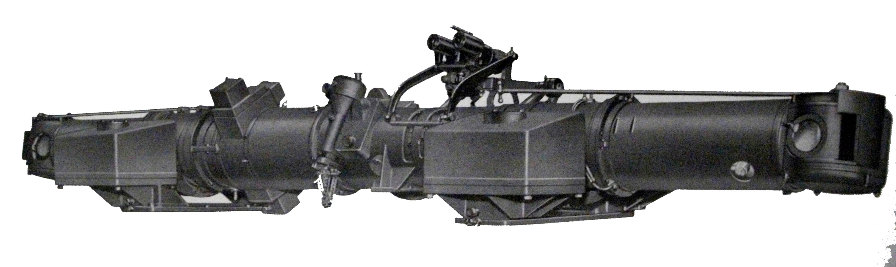
| Mk 3W rangefinder (Royal Navy) |
 |
| Type UR1 rangefinder on a MR24 mounting. The overall length is 12 feet. (Royal Navy) |
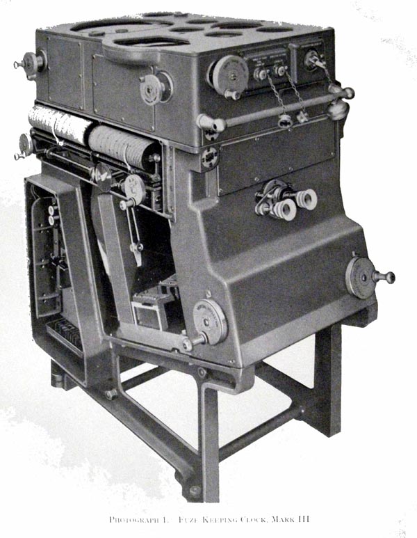 |
| Fuze Keeping Clock Mk 3. (Royal Navy) |
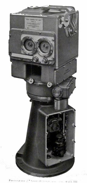 |
| Gyro Level Corrector for 285 system (Royal Navy) |
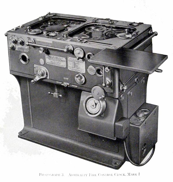 |
| Admiralty Fire Control Clock Mk I (Royal Navy) |
REFERENCE MATERIAL1) A complete 285 User Handbook can be found here . It comes courtesy of Lt Cdr Brain Witts MBE RN. Brian runs the Gunnery School Museum on Whale Island. The manual was photographed by Clive Kidd of the Collingwood Heritage collection and converted into a PDF file. It was then reduced in size from 250 mb to a more manageable 17 mb using an app called "PDF Squeezer". Lastly, it was OCRd via "Nuance PDF converter".
2) The technical handbook for the 285(M) is CB R 4221 (1) (A) and (B).
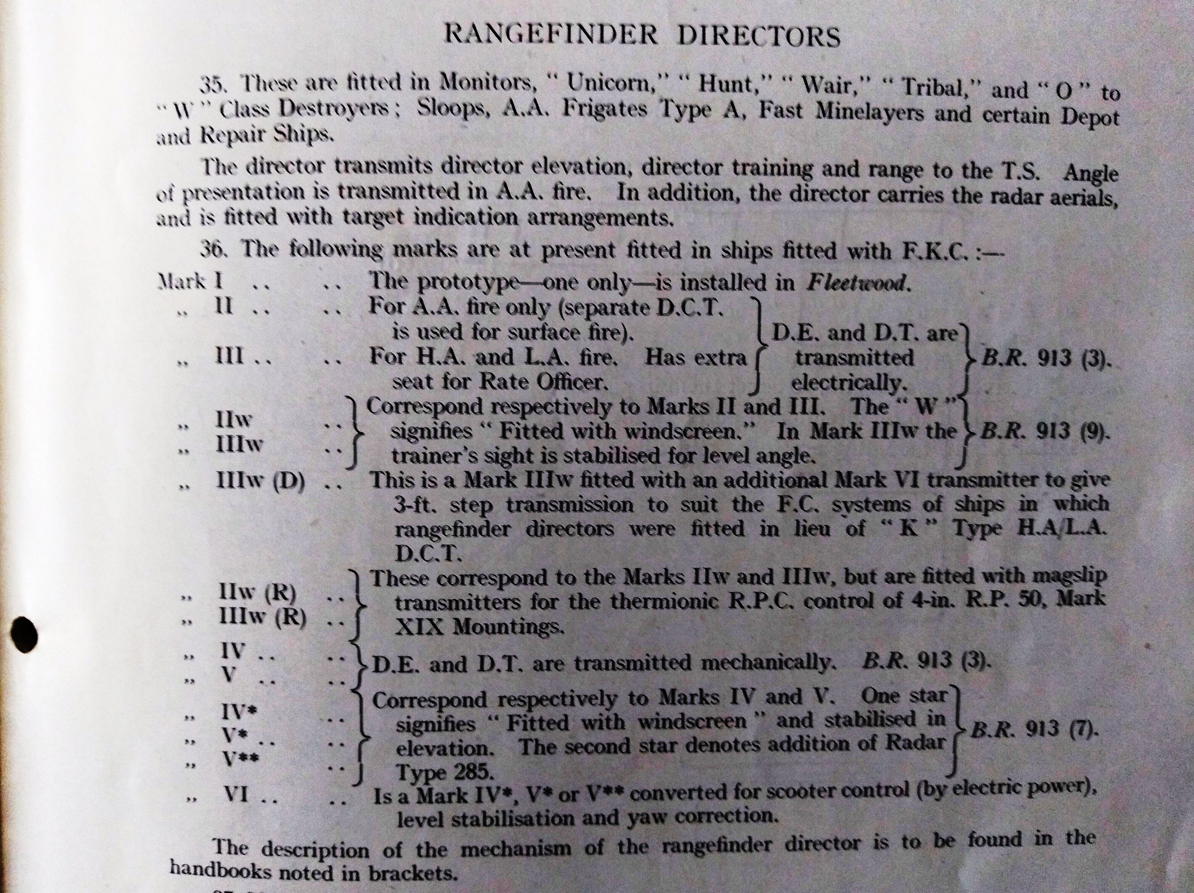
H90 is the Tech Handbook for 285 (P) and 285(Q)3) Listing of Rangefinding Directors.
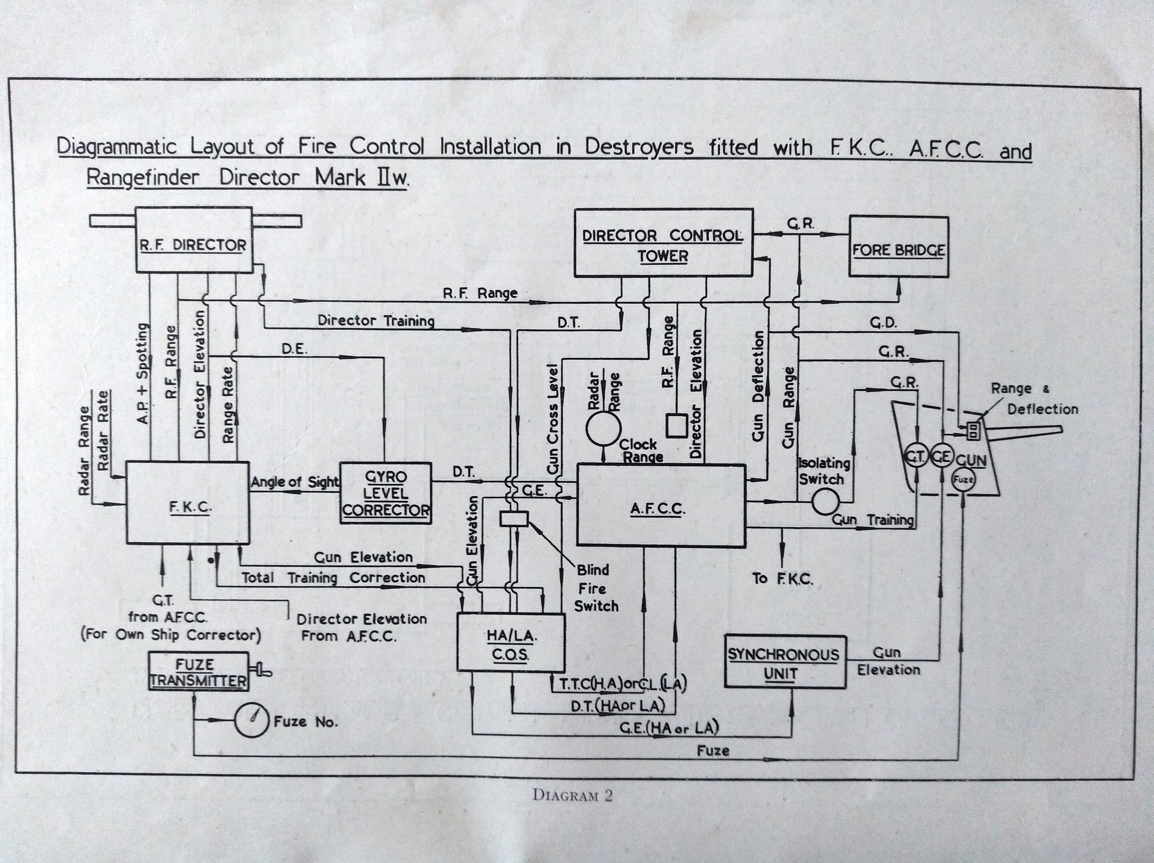
4) Block diagram of a FKC system with a Mk II rangefinder and Admiralty Fire Control; Clock. .
5) 285 application notes to HMCS HAIDA by Peter Marland
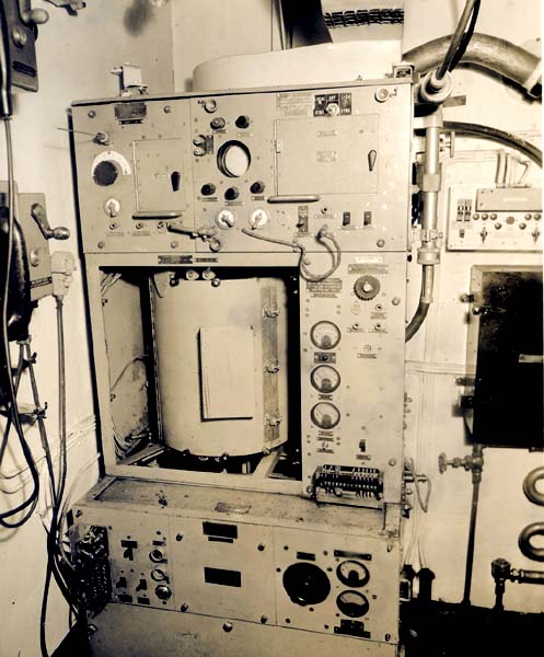 |
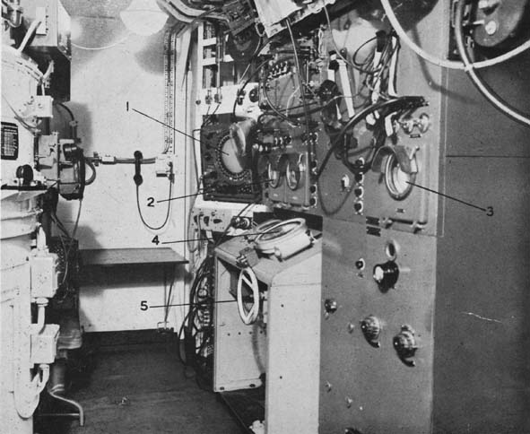
| Starboard bulkhead: 285 transmitter; supply board for outfit DPA (50 volt, 50 cycle, 3 phase). At very rightmost, a valve heating box for CV-13. (RCN photo # 1749-71) |
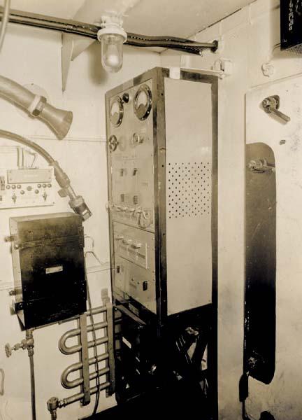 |
| Starboard bulkhead: Power board for outfit DPA; valve heating box.
After bulkhead (right side). Power supply board and motor starter for outfit DUA (180 volt, 500 cycle). (RCN photo # 1749-72) |
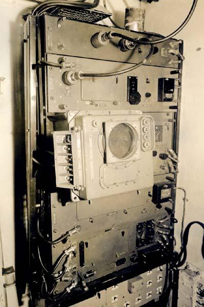 |
| After bulkhead: 285 receiver. (RCN photo # 1749-73) |
| The RCN photos in the this table came from the collection of the late John Rouey of Ottawa. |
Credits and References:1) The Threat to the S Band Marine Radar Frequency Allocation and the Necessity to Preserve It by John. H. Beattie, Journal of Navigation, no 53 (2000), pp 299-312.
2) Publication CB 4182/45 Radar Manual (Use of radar) from 1945.
3) Øyvind Garvik <oygarvik(at)online.no>
4) Le Musée Québecois de la Radio - Jacques Hamel, VE2DJQ
5) 268 manual extracts.
6) Peter Marland
Jan 6/25

